Why Division by Zero is a Bad Idea

A division by zero is primarily an algebraic question. The reasoning therefore follows the indirect pattern of most algebraic proofs:

What if it was allowed?

Then we would get a contradiction, and a contradiction is the greatest enemy of mathematical rigor. Many students tried to find a way to divide by zero once in their lifetime. To be honest: It is possible! We could allow it! However, that would come at a price. We had to give up other laws which we did not want to lose; most of all the fact that ##0## and ##1## are two different numbers. A division by zero often results in the equation ##1=0## which would make both of them pretty useless. But it also causes problems for other, often unexpected rules and laws that we do not want to give up.

Why division by zero is a bad idea as it implies …

10. 1=0.

This is the shortest argument of all:
$$
\dfrac{1}{0}=x \Longleftrightarrow 1=x\cdot 0=0
$$

9. All numbers are the same.

$$a\cdot 0=b\cdot 0 \Longrightarrow \dfrac{a}{0}=\dfrac{b}{0}=ba^{-1}\cdot\dfrac{a}{0}\Longrightarrow ba^{-1}=1\Longrightarrow a=b$$

8. Does numerator or denominator count?

A zero as a numerator makes a quotient vanish, and if the numerator and denominator are equal, then the quotient becomes one.

$$0=\dfrac{0}{x}=\dfrac{0}{0}=\dfrac{x}{x}=1$$

7. Division by zero equals zero.

$$1\cdot 0=2\cdot 0 \Longrightarrow \dfrac{1}{0}=\dfrac{2}{0}=\dfrac{1}{0}+\dfrac{1}{0}\Longrightarrow \dfrac{1}{0}=0$$

6. Division by zero equals infinity.

$$
\dfrac{1}{0}\stackrel{?}{=}\displaystyle{\lim_{n \to 0}\dfrac{1}{n}=\lim_{1/n \to \infty}\dfrac{1}{n}}=\infty
$$

5. Associativity breaks down.

$$\dfrac{1}{0}=x \Longleftrightarrow x\cdot 0=1 \Longleftrightarrow a=1\cdot a=(x\cdot 0)\cdot a \stackrel{(A)}{=}x\cdot(0\cdot a)=x\cdot 0=1$$

which is impossible for every ##a\neq 1.##

4. Distributivity breaks down.

$$\dfrac{1}{0}=x \Longleftrightarrow 1=x\cdot 0=x\cdot(1-1)\stackrel{(D)}{=}x\cdot 1-x\cdot 1= x-x= 0$$
which again contradicts ##1\neq 0.##

3. Infinity is not an option.

The difficulty by setting $$\dfrac{1}{0}:=\infty $$
is that infinity isn’t a number. Such a definition only shifts the ambiguity of a division by zero to the ambiguity of an infinitely large number. The problems are obvious:
$$
\begin{matrix}
\infty &+&\infty &=&\infty &\stackrel{?}{\Longrightarrow } &\infty &= &0\\
\infty &\cdot& \infty &=&\infty &\stackrel{?}{\Longrightarrow } &\infty &= &1
\end{matrix}
$$
And it goes on and on this way. Infinity isn’t well-defined. It is more like a large bin that swallows everything.

Let’s see whether L’Hôpital’s rule can help us,
$$
\displaystyle{\lim_{x \to 0}\dfrac{f(x)}{g(x)}=\lim_{x \to 0}\dfrac{f'(x)}{g'(x)}}
$$
where zeros and infinities on the left are explicitly allowed and only ##g'(0)\neq 0## and differentiability on the right are required. The condition on ##g'(0)## blocks the direct setting ##g’=0## or ##g=0.## If we set ##g'(x)=1## such that the condition holds, we get ##g(x)=x## and a denominator zero is not in sight. If we consider ##f(x)=x^{-1}## and ##f'(x)=-x^{-2}## we end up with
$$
\infty = \lim_{x \to 0}\dfrac{1}{x\cdot x}=\lim_{x \to 0}\dfrac{-1}{x^2\cdot 1}=-\infty
$$
which is obviously a problem. The missing differentiability at ##x=0## causes a contradiction.

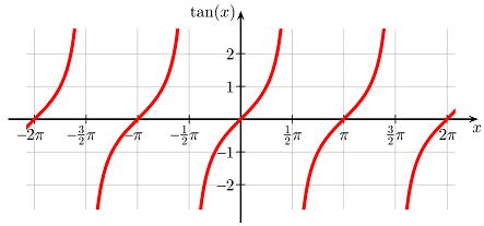
2. The geometric point of view.

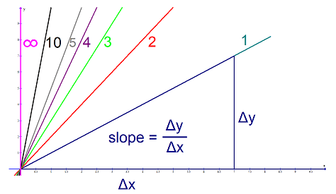
A slope of ##\dfrac{1}{0}## of a straight line is a vertical line, i.e. a line of infinite slope. We have already seen that infinity isn’t a good choice. It is the singularity of the tangent function at ##\pi/2## and we run into the same misery. Not only that we have a pole, we also have a sign change from ##-\infty ## to ##\infty ## depending on whether we approach from the left or the right.

1. ##\mathbf{0\not\in\mathbb{F}-\{0\}.}##

What looks like the most trivial argument is indeed the most subtle and my favorite one: ##0## as the neutral element of addition is not part of the multiplicative group ##\mathbb{F}^*=\mathbb{F}-\{0\}## of a field ##\mathbb{F}.## It has nothing to do with multiplication. The question of a multiplicative inverse of the neutral element of addition simply does not occur. It merely arises from our desire to consider fields as one set with two operations. However, they consist of two sets with two operations: ##(\mathbb{F},+)## and ##(\mathbb{F}^*,\cdot)##. The sets have many elements in common,
$$
\mathbb{F}^* \;\subset\; \mathbb{F},
$$
but they aren’t equal.

So why does the additive group contain the neutral element of multiplication, but the multiplicative group does not contain the neutral element of addition? This is primarily due to the way we construct number fields:
$$
\mathbb{N}\subset \mathbb{Z}\subset \mathbb{Q}\quad\text{ or }\quad\mathbb{N}\subset \mathbb{Z}\subset \mathbb{Z}_p=\mathbb{Z}/p\mathbb{Z}\,.
$$
We start with an additive group, discover a ring structure, and in case we get an integral domain, our ring allows a quotient field. Now, zero is a zero divisor, hence outside the set of elements we can construct quotients for; at least not by the usual method
$$
\dfrac{a}{b} \sim \dfrac{s}{t} \Longleftrightarrow a\cdot t= b\cdot s
$$
and as long as ##1\neq 0.## Rings do not necessarily contain the element ##1.## For example, all polynomials ##p(x)## with ##p(0)=0## build a ring without ##1.## On the other hand, ##\mathbb{Z}/n\mathbb{Z}## is only an integral domain, i.e. allows a quotient field, if ##n## is prime. These are the restrictions we have to deal with if we follow the constructional path from an additive group over a ring to a field. If we were to start with two different groups from scratch and search for a combination, then we would end up with free, direct, or semidirect products, which are different algebraic subjects.

Addition and multiplication in a field are only connected by the distributive laws inherited from its ring structure
$$
a\cdot (b+c)=a\cdot b+a\cdot c \quad\text{ and }\quad(a+b)\cdot c= a\cdot c+b\cdot c
$$
These two equations are the only ones where both operations meet. We have already seen that using them to define ##\frac{1}{0}## leads to ##1=0.## This cannot be a field anymore since ##1## would be a zero divisor and as such could not be part of the multiplicative group, which is a contradiction.

Extended Reals and Hyperreals

The extended real numbers are ##overline{mathbb{R}}=mathbb{R}cup {pm infty}.## They play a role in analysis as seen from a measure theoretical point of view, mainly to simplify statements about intervals or possible limits. Hewitt, Stromberg (Real and Abstract Analysis, GTM 25) define them as follows (bolding by me).

Definition: ##\infty ## and ##-\infty ## be two distinct objects, neither of which is a real number. The set ##\overline{\mathbb{R}}## is known as the set of extended real numbers. We make ##\overline{\mathbb{R}}## a linearly ordered set by taking the usual ordering in ##\mathbb{R}## and defining ##-\infty

The particular caution Hewitt, Stromberg take to avoid infinities being mistaken for numbers shows us that extended reals will not solve our problem to make ##\frac{1}{0}## a number. The extended real numbers are primarily a topological rather than an algebraic concept, and dividing points or solitons is hardly a promising approach.

When Newton and Leibniz performed their differential calculus with “fluxions” or “monads”, they used infinitesimal numbers, and Euler and Cauchy also found them useful. Nevertheless, these numbers were viewed skeptically from the beginning. As analysis was put on a rigorous basis by the introduction of the epsilon-delta definition of the limit and the definition of real numbers by Cauchy, Weierstrass, and others in the 19th century, infinitesimal quantities weren’t required anymore. However, Abraham Robinson showed in the 1960s how infinitely large and small numbers can be defined in a strictly formal way, opening up the field of nonstandard analysis with so-called hyperreal numbers ##\;{}^*\mathbb{R}.## [de.wikipedia.org: Hyperreal Numbers] 1)

The hyperreal numbers, a term introduced by Edwin Hewitt in 1948, satisfy the transfer principle, a rigorous version of Leibniz’s heuristic law of continuity. It is the central concept that makes nonstandard analysis at least analysis. It means that all true statements in real analysis, i.e. about ##\mathbb{R},## remain true in nonstandard analysis, i.e. about ##{}^*\mathbb{R}.## An example of how the hyperreals work is the derivative of a function
$$
f'(x)=st\left(\dfrac{f(x+\varepsilon )-f(x)}{\varepsilon }\right)
$$
where ##\varepsilon ## is an infinitesimal and ##st## is the standard part function that maps any hyperreal number to the nearest real number. This definition doesn’t need quantifiers anymore, and neither does it use the epsilontic of a limit. The transfer principle does not mean that real and hyperreal numbers behave the same, only that we do not lose what we already know. For example, we still have differentiation but ##{}^*\mathbb{R}## is not Archimedean anymore. Similarly, the casual setting ##\frac{1}{0}=\infty ## is invalid since the transfer principle applies and zero has no multiplicative inverse. The rigorous counterpart of such a calculation would be
$$
\dfrac{1}{\varepsilon }= \dfrac{\omega }{1} \text{ if }\varepsilon \neq 0
$$
where ##\varepsilon ## is an infinitesimal and ##\omega ## an infinite number. Thus, the transfer principle that we need to save what we already know about analysis, also prohibits us from making ##\frac{1}{0}## a number, even in the extended set of hyperreal numbers.

_____________

1) Details about hyperreal numbers can be found on the various language versions of Wikipedia or by searching for “hyperreal” among the Insight articles at PF.