The Slinky Drop Experiment Analysed

Figure 1: A slinky, the subject of the slinky drop experiment. Attribution: Roger McLassus. CC BY-SA

The slinky drop is a rather simple experiment. In its most basic form, it requires only a popular toy for children, a stable hand, and a keen eye. For a better view, using a modern smartphone to capture a video of the experiment also helps to capture the falling slinky. Apart from the commonly quoted result, Insight will discuss the evolution of the slinky shape during the drop using only high-school physics: mechanical equilibrium and the conservation of momentum.

What is The Slinky Drop Experiment?

The slinky drop experiment is exactly what it sounds like:

1. Support a slinky at one of its ends. Let the rest of it hang freely under gravity until it has reached equilibrium.
2. Let go of the slinky!
3. Observe how it falls under the influence of gravity and internal forces. Pay particular note to the motion of the lower end.

The result of the experiment is quite stunning and surprising to many. If you wish to experiment yourself before we go any further, stop reading now!

Results

Immediately after release, the lower slinky end remains motionless for some time. This lasts until the disturbance created by releasing the upper end reaches the lower end. If you did not have the means or will to experiment yourself, there is a popular video by Veritasium:

The explanation for the lower end remaining stationary is in the video, but we summarise it for completeness: While the segment of slinky just above the end remains stretched, it acts on the end part with the same force as before the drop. This is exactly the force required to balance gravity as the slinky was released from equilibrium. As a result, the lower part remains stationary until the disturbance reaches it. It just does not matter what happens higher up in the slinky until the disturbance passes.

Analyzing the Slinky Drop

While the explanation is uncontroversial, there is some ambiguity like the disturbance. Some sources seem to suggest that a regular compression wave travels down the slinky. However, there are several issues with such a model, including not matching the slinky shape during the fall very well. In some sense, this is great news! To truly understand such a wave we would have to derive and solve the wave equation for the slinky. This is a task that would be suitable for second or third-year students in university physics.

Instead of a regular compression wave and solving the wave equation, the physics of the slinky drop is relatively simple. Indeed, a pretty good model can be understood using the basic concepts of high school physics. The analysis below first introduces the setup of the mathematical framework. It then continues to discuss the equilibrium shape of the slinky and finally discusses the dynamics of the drop.

Setup

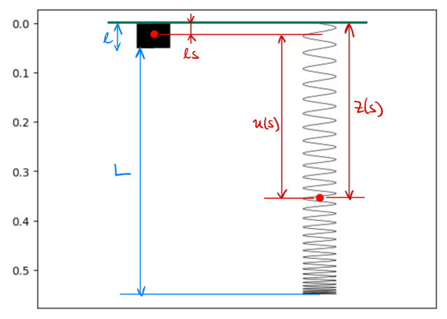
Figure 2: Setup of the slinky description. The left slinky has its rest length ##\ell## and the right one hangs under the influence of gravity. The red dot represents the same material point in both cases.

We model the slinky as an elastic spring of rest length ##\ell## and mass ##m##. We introduce a vertical coordinate ##z## such that the upper end of the slinky is held at ##z = 0## and the coordinate increases in the down direction. Furthermore, we introduce ##s## as a coordinate describing the fraction of the slinky above a particular point. In the absence of gravity, the slinky would be at rest. The position ##z(s)## of a point on the string is then: $$z(s) = \ell s$$ The position ##z(s)## when stretched is instead generally on the form $$z(s) = \ell s + u(s).$$ Here, ##u(s)## is the displacement from the rest position and it will be our focus from now on. A graphical representation of the setup is shown in Figure 2.

The Slinky in Equilibrium

According to Hooke’s law, the tension ##T(s)## in the slinky at string fraction ##s## is proportional to the strain ##u'(s)##. Mathematically, this implies that $$T(s) = \alpha u'(s),$$ with ##\alpha## being a constant. To find the equilibrium for the hanging slinky, we can now make a free-body diagram of the slinky part underneath ##s##.

Two forces are acting on this part: the force ##T(s)## due to tension and gravity. With the mass underneath ##s## being given by ##m(1-s)## and the forces balancing each other, we must have $$T(s) = \alpha u'(s) = mg(1-s).$$ Integrating this and using ##u(0) = 0## (as the upper end is fixed at ##z = 0##) leads to $$u(s) = \frac{mg}{\alpha} s\left( 1 – \frac s2\right) = 2Ls\left( 1 – \frac s2\right) \equiv u_0(s).$$ In the above the new constant ##L = u(1) = mg/2\alpha##, which is the total elongation of the slinky in equilibrium, has been introduced.

Two Sections of the Slinky

Once released, the upper part of the slinky starts falling immediately. The lower part remains stationary until the disturbance reaches it. The video capture of a dropping slinky suggests that the upper part moves as one, essentially in the slinky’s rest configuration, once the disturbance has passed. This suggests that the part above the disturbance front continuously collides inelastically with the next part of the slinky.

Describing the above mathematically, let ##s = \sigma(t)## be the position of the front of the disturbance a time ##t## after the drop. The slinky displacement ##u(s,t)## now also depends on ##t## and is on the form $$u(s,t) = u_0(\max(s,\sigma(t))).$$ In other words, the part ##s \sigma(t)## remains stationary.

The velocity of the slinky at ##s## for the part above ##\sigma(t)## takes the form $$v(t) = \frac{d}{dt} u_0(\sigma(t)) = \sigma'(t) u’_0(\sigma(t))  = 2L\sigma'(t)(1-\sigma(t)).$$ Correspondingly, the momentum of that part – and therefore also the total momentum of the slinky – is $$p = m\sigma v = 2mL\sigma’ \sigma(1-\sigma),$$ where we have suppressed the time dependence for readability.

The Slinky and Gravity

The only external force acting on the slinky during the drop is gravity. It acts with a total force ##mg## at all times. After time ##t##, the total momentum in the slinky is therefore ##p = mgt##. Equating the two expressions for the slinky momentum leads to $$\sigma’\sigma(1-\sigma) = \frac{gt}{2L}.$$ Integrating both sides with respect to ##t##, the relation between ##\sigma## and ##t## becomes $$\sigma^2 \left(\frac 12 – \frac \sigma 3\right) = \frac{gt^2}{4L}.$$

Finding a closed-form expression for ##\sigma(t)## requires finding the roots of a third-order polynomial. We will not do this here. However, only one of the roots will be in the range ##0 \leq \sigma(t) \leq 1##. As a curiosity, for small ##t## we find that $$\sigma(t) \simeq t \sqrt{\frac{g}{2L}}.$$ Consequently, $$v(0) = 2L \sigma'(0) = \sqrt{2Lg}$$ meaning that the disturbance moves at a non-zero speed from the beginning of the drop.

Illustrating the Drop

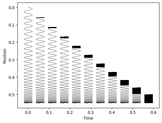
Figure 3: The model prediction for the shape of the slinky during the drop at different times. Units are arbitrary and the last slinky shows the fully contracted slinky. The model prediction for later times is this slinky simply continues to fall.

Luckily, a computer can easily find the root for us to illustrate the slinky shape during the drop as shown in Figure 3. From the figure, we can also see the characteristic effect of the slinky bunching up from the top as it continues to fall.

We can also note that the disturbance reaches ##\sigma(t) = 1## when $$t = \sqrt{\frac{2L}{3g}}.$$ It is easy to verify that this is exactly the time required for the center of mass to fall past the lower end of the slinky.

Concluding Remarks

As with any mathematical model of a physical system, the model above has its limitations. Although it provides a pretty good fit to the slinky evolution in general, it also fails to reproduce some effects. For example:

• The full slinky motion is described as one-dimensional. A real slinky will inevitably also move in the horizontal direction. The real collisions are never truly one-dimensional. This is particularly noticeable towards the end of the drop.
• The inelastic collisions between the upper and lower parts of the string are rather simplistic. While it does give a decent description of the slinky, it will not occur as abruptly. In this sense, the model is rather coarse.

Note that what is described here is a disturbance that:

1. Moves faster than the characteristic wave speed in the slinky. (This can be checked, but is more involved so we leave this out.)
2. Has an abrupt change in the density of the slinky windings as the disturbance passes.

These characteristics are the characteristics of a shock wave rather than a compression wave propagating at the local wave speed. Trying to use the wave equation to describe the real slinky evolution is therefore doomed to failure.

Additional Reading and References

The exposition above closely follows the work of Unruh:

Unruh uses different notation and conventions, but the essentials are the same.

The slinky drop experiment was first described by Calkin:

Further analyses with more intricate modeling can be found in the following papers (a selection):

For an example of suggested related educational activities, see:

• C. Berggren, P. Gandhi, J. A. Livezey, R. Olf, A Tale of Two Slinkies: Learning about Model Building in a Student-Driven Classroom, The Physics Teacher 56 134 (2018)