Exploring the Multifaceted Nature of Complex Numbers

Abstract

Why do we need yet another article about complex numbers? This is a valid question and I have asked it myself. I could mention that I wanted to gather the many different views that can be found elsewhere – Euler’s and Gauß’s perspectives, i.e. various historical views in the light of the traditionally parallel development of mathematics and physics, e.g. the use of complex coordinates in kinematics, the analytical or topological views, e.g. the Radish or the mysterious Liouville’s theorem about bounded entire functions that are already constant, or the algebraic view that led to the many non-algebraic proofs of the fundamental theorem of algebra. The complex numbers have so many faces and appear in so many contexts that I could as well have written a list of bookmarks. All of that is true to some extent. The real reason is, that I want to break the automatism of the association of complex numbers with, and the factual reduction to points in the Gaußian plane
$$
\mathbb{C}=\{a+i b\,|\,(a,b)\in \mathbb{R}^2\}\neq \mathbb{R}^2.
$$
We need two dimensions to visualize complex numbers but that doesn’t make them two-dimensional. They are a one-dimensional field in the first place, i.e. a single set of certain elements that obey the same axiomatic arithmetic rules as the rational numbers do. They are one set that is not just a plane! The reason they exist and bar us from visual access is finally a tiny positive distance we can see.

The Algebraic View

Let ##\mathbb{F}## be a field of characteristic zero with an Archimedean ordering. This is algebra talk. A field means that we can add, subtract, multiply, and divide the way we are used to. Characteristic zero means, that
$$
1+1+ \ldots + 1 \neq 0
$$
no matter how many ones we add. Don’t laugh, you are – right now – using a device that has ##1+1=0## as its most fundamental law! An Archimedean ordering only means

$$
\forall \;a\in \mathbb{F} \;\exists \; n \in \mathbb{N}\, : \,n>a.
$$
And once again, don’t laugh, some fields contain the rational numbers and are not Archimedean. For the sake of simplicity, imagine ##\mathbb{F}=\mathbb{Q}## or ##\mathbb{F}=\mathbb{R}.## The following algebraic constructions work with rational numbers, too, i.e. the algebraic perspective does not require real numbers. We can have the algebraic closure first and the topological closure next, or vice versa.
$$
\begin{matrix}&&\overline{\mathbb{Q}}[i]&&\\
&\nearrow_{alg.} && \searrow^{top.} &\\
\mathbb{Q}&&&&\mathbb{C} \\
&\searrow^{top.} && \nearrow_{alg.} &\\
&&\mathbb{R}&&
\end{matrix}
$$
The central observation is that the polynomial ring ##\mathbb{F}[x]## is an integral domain and a principal ideal domain, i.e. any ideal in ##\mathbb{F}[x]## is already generated by a single polynomial. The reason for this is that ##\mathbb{F}[x]## is an Euclidean ring where we can perform a long division with the polynomial degree as the quantity decreases in the process. It is the size of the remainder that decreases in the usual process of the Euclidean algorithm. The size of polynomials is their degree.

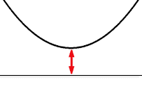
The availability of the Euclidean algorithm, however, has far-reaching consequences. The possibility of dividing polynomials allows the distinction between polynomials that have factors and those which do not. The latter are called irreducible polynomials. The tiny distance ##d\in \mathbb{F}_{>0}## with the red arrow in the image above guarantees that
$$
x^2+d
$$
is an irreducible polynomial over ##\mathbb{F}.## We cannot write it as a product of polynomials of degree one. A typical algebraic scheme of proof would be:

Assume ##x^2+d=(x+a)(x+b)=x^2+(a+b)x+ab.## Then ##a+b=0## and ##ab=-a^2=d.## Therefore ##x^2+d=x^2-a^2=(x-a)(x+a).## This polynomial has two zeros at ##x=a## and ##x=-a,## or one zero in case ##a=0.## But the image shows that ##x^2+d## does not cross the line ##y=0,## i.e. the polynomial has no zeros. This contradiction means that ##x^2+d## is indeed irreducible.

Since ##\mathbb{F}[x]## is a principal ideal domain, the irreducible polynomial ##x^2+d## is automatically a prime element, and it generates a prime ideal ##\bigl\langle x^2+d \bigr\rangle ## that is automatically a maximal ideal, so that the factor ring

$$
\mathbb{F}[x]/\bigl\langle x^2+d \bigr\rangle = \mathbb{F}\left[ \sqrt{-d}\right]
$$

is automatically a field. Now that ##x^2+d## is made zero, we can identify ##x## with ##\sqrt{-d}## and
$$
x^2+d=\left(x-\sqrt{-d}\right)\cdot \left(x+\sqrt{-d}\right)\equiv 0
$$
has two new zeros ##\pm \sqrt{-d}##, however, outside of ##\mathbb{F}.## If ##d=1## and ##\mathbb{F}=\mathbb{R}## then we call this field the complex numbers
$$
\mathbb{R}[x]/\bigl\langle x^2+1 \bigr\rangle =\mathbb{R}\left[ \sqrt{-1}\right]=\mathbb{C}.
$$

The Arithmetic Rules

When I said that complex numbers and rational numbers obey the same axiomatic rules, I referred to the fact that both have an additive and a multiplicative group connected by the distributive laws as in any field. Derived rules, abbreviations, or interpretations are no longer automatically true, simply because ##z^2\geqq 0## is no longer true. This has consequences. The most prominent example is
$$
-1=\sqrt{-1}\cdot \sqrt{-1} \neq \sqrt{(-1)\cdot (-1)}=\sqrt{1}=1.
$$
The derived rule ##\sqrt{a\cdot b}=\sqrt{a}\cdot \sqrt{b}## for real numbers does not hold anymore. But how can we know which ones still hold and which ones do not without searching for a proof in every single case? Well, we could learn what is written in this article (Things Which Can Go Wrong with Complex Numbers) or use the definition we just learned. This means that we identify ##i=\sqrt{-1}## with the indeterminate ##x## of the real polynomial ring ##\mathbb{R}[x]## and establish the law ##x^2+1 \equiv 0.## The equation above becomes
$$
x\cdot x \equiv -1 \neq 1=\sqrt{1}=\sqrt{(-1)^2}
$$
We can write the equations on the right because ##(-1)^2\geqq 0## for real numbers, however, ##x^2\ngeqq 0## in ##\mathbb{R}[x]/\bigl\langle x^2+1 \bigr\rangle ,## and ##\sqrt{x^2}## isn’t even defined in ##\mathbb{R}[x]/\bigl\langle x^2+1 \bigr\rangle .## Hence, the algebraic view on complex numbers can prevent us from making arithmetic mistakes. All we have is a field of scalars of characteristic zero. Any functions like square roots, logarithms, etc. have to be reconsidered. ##\mathbb{C}## doesn’t even have an Archimedean ordering any longer.

Reconsidered Analysis

As much as the algebraic view can help to avoid arithmetic mistakes, as much does it have a significant disadvantage if we want to perform analysis on ##\mathbb{R}[x]/\bigl\langle x^2+1 \bigr\rangle .## It is inconvenient and ambiguous since we will need polynomials in their analytical meaning as functions, too. Hence even if I may not like the point of view as points in the Gaußian plane, we have to consider the complex numbers as real vectors, too. I’m not too fond of it because it supports the impression that complex numbers are only real vectors. They are not, they are scalars, and especially complex analysis is full of examples where this fact is important. Nevertheless, we need help in the form of visualization and we can only see the real world.

The Real Vector Space

\begin{align*}
\mathbb{C}&=\mathbb{R}[x]/\bigl\langle x^2+1 \bigr\rangle = \{p(x)=a+bx\,|\,(a,b)\in \mathbb{R}^2 \wedge x^2+1\equiv 0\}  \\[12pt]
\mathbb{C}& =\{z=a+i b\,|\,(a,b)\in \mathbb{R}^2\}=\mathbb{R} \oplus i\cdot \mathbb{R}
\end{align*}
are both representations of the complex numbers as primarily a two-dimensional real vector space with the – in my opinion a bit hidden – additional property ##x^2=-1,## resp. ##i^2=-1.## The two components ##(a,b)## of a complex number ##z## are called
\begin{align*}
a&=\mathfrak{Re}(z)\text{, real part of }z\text{ and}\\[6pt]
b&=\mathfrak{Im}(z)\text{, imaginary part of }z.
\end{align*}
They are the Cartesian coordinates in the Gaußian plane. The corresponding polar coordinates $$z=r\cdot e^{i \varphi }=r\cdot (\cos \varphi +i \sin \varphi )$$ which are very important in physics but often a bit neglected in mathematics are called
\begin{align*}
r&=\sqrt{a^2+b^2}\text{, the absolute value of }z\text{ and}\\[6pt]
\varphi &= \sphericalangle (a,b)\text{, the argument of }z.
\end{align*}
The absolute value is the Euclidean distance from the origin of the Gaußian plane, and the argument is the direction to ##(a,b)## measured as an angle from the positive real axis. However, the additional arithmetic law

$$
(i\cdot \mathbb{R})\cdot (i\cdot \mathbb{R}) \subseteq \mathbb{R}
$$
other than in an ordinary real Euclidean vector space makes a crucial difference and should not be forgotten. I think the connection between real and complex numbers can best be memorized by a formula many mathematicians consider the most beautiful equation of all
$$
e^{i\cdot\pi}+1=0 .
$$

The Radish

The formula ##(i\cdot \mathbb{R})^2 \subseteq \mathbb{R} ## should better be written as

$$
( i \cdot \mathbb{R})^{2n} \subseteq \mathbb{R}\, ,\,( i \cdot \mathbb{R})^{2n+1} \subseteq i \cdot \mathbb{R}\, , \,n \in \mathbb{Z}
$$
to note that we could switch as often as we want between the two dimensions by a simple multiplication. It reflects the more general case of multiplication which becomes obvious in polar coordinates
$$
\left(r\cdot e^{i \varphi }\right)\cdot \left(s\cdot e^{i \psi }\right) = (rs)\cdot e^{i(\varphi + \psi )}.
$$
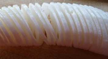
Multiplication is a rotation of directions and we can all of a sudden count how often we pass the gauge line, the positive real axis. We have a radish.

This picture is particularly important for the complex logarithm function since
$$
\log z = \log \left(re^{i \varphi }\right)= (\log r) + i \varphi
$$
does not tell us on which slice ##n ## of the radish we are. We only know it up to full rotations
$$
\varphi = \varphi_0 + 2n\pi .
$$
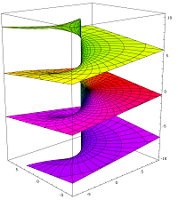
The range ##\varphi_0 \in (-\pi,\pi]## is called the principal value, and the corresponding slice of the radish ##n=0## is called the principal branch. The radish is cut along the negative real axis and the origin is called branch point. Mathematicians prefer to speak of branches instead of radish slices but the picture helps to understand what is going on. An official picture of the radish would be

The Functions

Complex function theory goes far beyond our subject of complex numbers. We have just seen in the example of the complex logarithm that winding numbers and poles play a central role. Note that ##\log (0)## is a pole and no value can be attached to it. One could call complex function theory Cauchy’s winding and residue calculus because of the residue theorem, a generalization of Cauchy’s integral theorem and integral formula,
$$
\oint_\gamma f(z)\,dz=2\pi i\cdot \sum_{\substack{\text{poles}\\[2pt]p_k}} \underbrace{\operatorname{Ind}_\gamma (p_k)}_{\substack{\text{windings }\\[3pt] \text{around }p_k\text{ of} \\[3pt] \text{integration path }\gamma }}\cdot \underbrace{\operatorname{Res}_{p_k}(f)}_{\substack{\text{coefficient }-1\text{st}\\[3pt] \text{ in the Laurent }\\[3pt] \text{series of }f\text{ at }p_k}}.
$$
But this isn’t the only property of complex functions we are not used to from real calculus. Any complex function that is complex differentiable is already smooth, i.e. it is infinitely often complex differentiable. And if it is in addition bounded, then it is already constant (Liouville’s theorem):
\begin{align*}
\left|f'(z)\right|&=\left|\dfrac{1}{2\pi i}\oint_{\partial U_r(z)}\dfrac{f(\zeta)}{(\zeta-z)^2}d\zeta\right|\leqq \dfrac{1}{2\pi}\cdot 2 \pi r \cdot \dfrac{C}{r^2}\stackrel{r\to \infty }{\longrightarrow }0.
\end{align*}
We can write every complex function as
$$
f(z)=f(a+ib)=\mathfrak{Re}(f(z))+\mathfrak{Im}(f(z))
=u(a,b)+i\cdot v(a,b)
$$
with two real functions ##u,v\, : \,\mathbb{R}^2\rightarrow \mathbb{R}.## I have learned that the complex function ##f## is differentiable if the real functions ##u,v## are differentiable and the Cauchy-Riemann equations hold
$$
\dfrac{\partial u}{\partial a}=\dfrac{\partial v}{\partial b}
\ ,\ \dfrac{\partial u}{\partial b}=-\dfrac{\partial v}{\partial a}.
$$
As true as it is, it is in my mind an insufficient perspective. I like Weierstraß’s decomposition formula
$$
f(z)=f(a) + D_a(f) \cdot (z-a) +o(z-a)
$$
to define differentiability. It displays all necessary aspects and puts the limit where it belongs, into the remainder term ##o(z-a).## Differentiability at a point ##a\in \mathbb{C}## – a local property(!) – is then the existence of the ##\mathbb{C}##-linear function ##f'(a)=D_a(f),## the derivative in ##a##. The emphasis on ##\mathbb{C}##-linearity is crucial here. After all, it is the reason behind the Cauchy-Riemann equations and why I prefer to consider complex numbers as a field of scalars rather than a real vector space with extras. The clumsy definition by real differentia-
bility plus Cauchy-Riemann equations are all contained in the simple requirement that ##D_a(f)## is ##\mathbb{C}##-linear, see [3].

FTA And The Two Closures

The fundamental theorem of algebra (FTA), that every complex polynomial ##f(z)## of degree at least one has at least one zero, can be proven quite elegantly with the help of Liouville’s theorem. Since
$$
\lim_{n \to \infty}\inf_{|z|=n}|f(z)|=\infty
$$
there is a real number ##r## such that ##|f(0)|\leqq |f(z)|## for all ##z\in \{z\in \mathbb{C}\,|\,|z|>r\}##. Since ##f## and in addition to that ##|f|## is continuous, it takes a minimum, say at ##z_0,## in the compact disc ##D=\{z\in \mathbb{C}\,|\,|z|\leqq r\}## according to Weierstraß’s theorem about the minimum and maximum. This means that
$$
0\leqq C:=|f(z_0)|\leqq |f(z)|\;\text{ for all }z\in D.
$$
This value is already a global minimum per construction. If ##C>0## then
$$
f^{-1}\, : \,z\longmapsto \dfrac{1}{f(z)} \leqq \dfrac{1}{C}
$$
would be a holomorph, bounded function defined on ##\mathbb{C}.## Liouville’s theorem now says that ##f^{-1}## has to be constant, i.e. ##f## is also constant, contradicting our choice of the polynomial ##f## of at least degree one. Thus ##C=0=f(z_0)## and we have found a zero ##z_0## of ##f.\; \square ##

Note that we used pure analytical tools to prove the fundamental theorem of algebra. We also needed both closures of ##\mathbb{C}.## What does that mean? A sequence ##(a_n)_{n\in\mathbb{N}}## is called a Cauchy sequence if
$$
\displaystyle{\lim_{n,m \to \infty}|a_n-a_m|=0}.
$$
Unfortunately, this does not mean that ##\displaystyle{\lim_{n \to \infty}a_n}## exists. If we define for instance
$$
a_1=2\;\text{ and }\; a_{n+1}=\dfrac12 \left(a_n+\dfrac{2}{a_n}\right)\text{ for }n\in \mathbb{N}
$$
we get a decreasing Cauchy sequence of rational numbers converging to ##\sqrt2.## But this limit does not exist in ##\mathbb{Q}.## To make all limits available, we topologically complete the rational numbers by adding all possible limits of Cauchy sequences obtaining the real numbers. The existence of ##z_0,## i.e. the existence of a Cauchy limit ##z_0## in the proof above has been provided by a topological argument about real numbers hidden in Weierstraß’s theorem.

The topological closure is not the only closure that we need. If we think about our first example ##f(x)=x^2+d \;(d>0),## then we have a parabola – a polynomial of degree two – that does not have a real zero. It does not cross the real axis. Completion of the square
$$
0=x^2+px+q=\left(x+\dfrac{p}{2}+\sqrt{\dfrac{p^2}{4}-q}\right)\cdot \left(x+\dfrac{p}{2}-\sqrt{\dfrac{p^2}{4}-q}\right)
$$
is a standard method to find the zeros of quadratic polynomials. This means for our original example
$$
0=x^2+d=\left(x+\sqrt{-d}\right)\left(x-\sqrt{-d}\right)=\left(x+i \cdot \sqrt{d}\right)\left(x-i \cdot \sqrt{d}\right)
$$
that we have two complex roots ##\pm i\cdot \sqrt{d}.## In general, we have the situation that
$$
\sqrt{\dfrac{p^2}{4}-q}=\dfrac{1}{2}\sqrt{p^2-4q}=\begin{cases}
\dfrac{1}{2}\sqrt{p^2-4q} \in \mathbb{R}&\text{ if }p^2>4q\\[6pt]
\quad \quad \quad 0&\text{ if }p^2=4q\\[6pt]
\dfrac{i}{2}\sqrt{4q-p^2}\in i\mathbb{R}&\text{ if }p^2
\end{cases}
$$
decides whether we have two real, one real, or two complex solutions. The term ##\Delta=p^2-4q## is called the discriminant of ##x^2+px+q.## If we have a real, monic (highest coefficient is one) polynomial ##f(x)## of degree ##2n+1## then
$$
\lim_{x \to -\infty}f(x)=-\infty \;\text{ and }\;\lim_{x \to +\infty}f(x)=+\infty
$$
and by topological completeness of ##\mathbb{R}## we have a real zero ##x_0\in \mathbb{R}## and may write
$$
f(x)=g(x)(x-x_0) \;\text{ with }\;\deg g(x)=2n.
$$
It can be proven now that the zeros of polynomials of even degree always appear as conjugates
$$
\left(-\dfrac{p}{2}\right) + \left(\dfrac{\sqrt{\Delta}}{2}\right) \;\text{ and }\;\left(-\dfrac{p}{2}\right) – \left(\dfrac{\sqrt{\Delta}}{2}\right).
$$
This means that the example with the parabola is a typical one, and we only have to attach ##\pm i\cdot\sqrt{d}## to the real numbers to decompose any polynomial into linear factors. Since ##sqrt{d}in mathbb{R},## it is sufficient to attach ## i ## as the formal solution to the quadratic polynomial equation ##x^2+1=0.## This formal symbol is the reason why we first considered
$$
\mathbb{C}=\mathbb{R}[x]/\bigl\langle x^2+1 \bigr\rangle =\mathbb{R}[i].
$$
The field extension ##\mathbb{R}\subseteq \mathbb{R}[ i ]## is called the algebraic closure of ##\mathbb{R}.## Which closure comes first and which one next doesn’t matter as long as we arrive at the field of complex numbers. The algebraic closure necessary to find all polynomial zeros is even better hidden in the above proof of the FTA than the topological closure. It is ultimately hidden in Cauchy’s integral formula that is used to prove Liouville’s theorem. For those who prefer an axiomatic description of the complex numbers, see [5] which cites Spivak’s calculus book. For a formal algebraic construction of real and complex numbers, I recommend van der Waerden’s book on Algebra [7].

Sources