

Introduction
The concept of a group is as simple as it gets: a set with a binary operation like addition and a couple of natural laws like the requirement that the order of two consecutive operations does not matter: ##(1+2)+3=1+(2+3).## That’s it. The concept of a group is so simple that I still wonder why it wasn’t part of my syllabus at school. And, yet, it covers such different sets like the integers, the hours that the big hand counts, the symmetries in a crystal, the Caesar cipher, or a light switch which is the basis of our electronic world. However, few requirements allow many additional, more specific refinements. In the case of groups, we arrive at strange-sounding results like the fact that the largest finite, and simple, sporadic group has
$$
808017424794512875886459904961710757005754368000000000
$$
many elements. This article is meant to shed some light on the betweens of a light switch and a group with more than ##8\cdot 10^{53}## elements that mathematicians dare to call simple. At least, they also call it the monster group, and the second largest finite, simple, sporadic group with its
$$
4154781481226426191177580544000000
$$
many elements baby monster group. And to be honest, even the simple fact that they found them is still a mystery to me.
This article explains fundamental concepts and only lists the mysterious results. It is meant as an introduction to group theory rather than a treatment of the many special areas into which group theory has branched out. Many statements especially in the sections about examples and structures can be verified by the readers if they wish to practice typical conclusions in group theory.
Definitions
A group has only one binary operation, regardless of whether there can be defined more than one binary operation on the underlying set. This unique operation can be written by a plus sign, a dot, or a small circle. The plus sign is usually reserved for groups with a symmetric operation, in which case we call the group commutative or abelian. Groups are not necessarily commutative. The preferred sign for the operation of arbitrary groups is the dot, which is also left out as usual: ##(a,b)\mapsto ab.## If we look up the definition of a group then we will probably find three requirements. The order of two consecutive operations must be irrelevant, called associativity, i.e. ##a(bc)=(ab)c,## there has to be a neutral element ##e## such that ##ae=ea=a,## and inverse elements ##a^{-1}## such that ##a^{-1}a=aa^{-1}=e.## This sounds more artificial than it is. An alternative and equivalent definition mimics the transition from non-zero integers to non-zero rational numbers. A group is a set with a binary, associative operation such that the equations ##ax=b## and ##xa=b## can always be solved. That’s what we did in the transition from integers to rationals: we made ##3x=2## solvable. The transition from natural numbers to integers for addition was accordingly: we made ##3+x=2## solvable. These solvability conditions guarantee a neutral element as the solution to ##ax=a,## and inverse elements as solutions to ##ax=e.## A group is therefore not only a very basic concept, groups also occur naturally as the fundamental structure of our number systems. The number of elements in a group ##G## is called the order of ##G## noted as ##|G|.## The notation is particularly important for finite groups, i.e. when ##|G|## is a positive integer. A notation ##|\mathbb{Z}|=\aleph_0## is rarely used.
Examples, Card Decks, and Caesar Ciphers
The additive group ##\left(\mathbb{Z},0,+\right)## of integers and the multiplicative group ##\left(\mathbb{Q},1,\cdot\right)## of non-zero rational numbers are both infinite. The trivial group ##\left(\{e\},e,\cdot\right)## is the smallest possible group. It consists only of the neutral element. We can create a finite group of any order if we take the set ##\{e,a,a^2,\ldots,a^{n-1}\}## and define ##a^n=e.## These groups are called cyclic. And we use them every day! A light switch with ##0=\text{OFF}## and ##1=\text{ON}## is such a group of order two, and our electronic devices are based on that principle. A bit is either ##0## or ##1## and using a light switch twice results in a neutral state as if we didn’t switch it. The hours of a day build a cyclic group of order twelve or twenty-four depending on what you call a day. These examples are usually written as additive groups since we add hours to circle a watch. However,
$$
\{e,a,a^2,\ldots,a^{n-1}\}\text{ and }\{0,1,\ldots ,n-1\}
$$
are the same group; written multiplicatively on the left and additively on the right. If we divide integers with remainder, i.e. we write ##N:n## as ##N= q\cdot n + r ,## then the set of possible remainders ##r## of a division by ##n## is the cyclic (additive) group with ##n## elements. These groups play a central role in number theory and cryptology. We write
$$
N\equiv r\pmod{n}
$$
and identify all numbers with their remainder. The group elements are thus equivalence classes represented by their remainder. The groups are finite, abelian, and cyclic, noted as ##\mathbb{Z}_n.## For instance ##n=5## results in the five elements of possible remainders
\begin{align*}
[0]&=\overline{0}=\{\ldots,-10,-5,0,5,10,\ldots\}\\
[1]&=\overline{1}=\{\ldots,-9,-4,1,6,11,\ldots\}\\
[2]&=\overline{2}=\{\ldots,-8,-3,2,7,12,\ldots\}\\
[3]&=\overline{3}=\{\ldots,-7,-2,3,8,13,\ldots\}\\
[4]&=\overline{4}=\{\ldots,-6,-1,4,9,14,\ldots\}
\end{align*}
The usual notation is to omit overlining or brackets and to simplify it by ##[a]=\overline{a}=a## since we usually only consider the representatives ##0,1,\ldots,n-1## of each equivalence class. However, we have to keep in mind that even if we write them as numbers, they are just representatives of entire sets.
We can also multiply remainders, so the set ##\mathbb{Z}_n## carries an additional commutative ring structure. This means, we have additionally to addition a commutative multiplication on ##\mathbb{Z}_n## that obeys the distributive law
$$
a\cdot (b+c)=a\cdot b+ a\cdot c
$$
Of course, we need to distinguish both operations in the case we speak about the ring structure. The multiplicative structure without the additive neutral element ##0## is again a group if and only if ##n## is prime. Generally, elements with a multiplicative inverse element are called units. Bézout’s identity provides an equation
$$
\operatorname{gcd}(a,n)=(a,n)=r\cdot a + s\cdot n
$$
so that ##r\cdot a\equiv 1\pmod{n}## in the case of coprime numbers ##a,n.## Hence, the units of the ring structure on ##\mathbb{Z}_n## are precisely the coprime elements. They build the multiplicative group ##\left(\mathbb{Z}_n^\times,\cdot\right)## of units of the ring ##\mathbb{Z}_n.##
The famous Caesar cipher is based on the cyclic group with twenty-three elements, an encryption the Romans used. All letters are numbered and shifted by a secret number ##k,## i.e.
\begin{align*}
\text{encrypt}_k(C)&=C+k\pmod{23}\longrightarrow S\\
\text{decrypt}_k(S)&=S-k\pmod{23}\longrightarrow C
\end{align*}
where ##C## is a letter of the clear text message and ##S## is the decoded secret letter. Both sides are supposed to know the value ##k.##
Finite cyclic groups do not only occur in the relatively simple, and not very secure Caesar cipher but also in many other often error-correcting codes, and the RSA encryption scheme.
The smallest non-cyclic group has four elements ##\{e,a,b,ab\}## and is the symmetry group of a proper (non-square) rectangle.
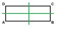 \begin{align*}
\left(A,B,C,D\right)&\stackrel{e}{\longrightarrow } \left(A,B,C,D\right)\\
\left(A,B,C,D\right)&\stackrel{a}{\longrightarrow } \left(B,A,D,C\right)\\
\left(A,B,C,D\right)&\stackrel{b}{\longrightarrow } \left(D,C,B,A\right)\\
\left(A,B,C,D\right)&\stackrel{ab}{\longrightarrow } \left(C,D,A,B\right)\\
\end{align*}
This group is called Klein Four Group ##V_4##. Instead of describing it by its Cayley table of all group multiplications between its abstract elements,
$$
\begin{array}{ccc}
\begin{array}{c||c|c|c|c|}
\cdot &e & a & b & ab\\
\hline
\hline e&e & a & b & ab\\
\hline a&a & e & ab & b\\
\hline b&b & ab & e & a\\
\hline ab&ab & b & a & e\\
\hline
\end{array} &
\text{ or shorter }&
\begin{array}{|c|c|c|c|}
\hline e & a & b & ab\\
\hline a & e & ab & b\\
\hline b & ab & e & a\\
\hline ab & b & a & e\\
\hline
\end{array}
\end{array}
$$
we described the group elements as functions and what they did to a rectangle. Group elements are no longer numbers but symmetries, i.e. functions of the vertices. This point of view opens the door to an entirely new world of groups and the class of symmetry groups. Let us consider a deck of poker cards. It comes in a certain order if it is new and every shuffle creates a new order.
$$
80658175170943878571660636856403766975289505440883277824000000000000
$$
possible results of a shuffle and naming the shuffled elements by their card values is quite inconvenient. Mathematicians shuffle the numbers ##\{1,2,\ldots,n\}## instead and write the group of all possible shuffling processes as ##\operatorname{Sym}(n)## with ##1\cdot 2\cdots n=n!## elements. A group element is thus a permutation of the ordered sequence ##(1,2,\ldots,n)## into another ordering ##(a_1,a_2,\ldots,a_n)## written as
$$
\begin{pmatrix}1&2&\ldots&n\\a_1&a_2&\ldots&a_n\end{pmatrix}.
$$
The group operation is shuffling them again, i.e. the consecutive application of two permutations. This leads us to ##\operatorname{Sym}(3),## the smallest example of a non-abelian group, i.e. a group where ##ab\neq ba## for some of its elements:
$$
\begin{pmatrix}1&2&3\\2&1&3\end{pmatrix}\circ \begin{pmatrix}1&2&3\\3&1&2\end{pmatrix}=
\begin{pmatrix}1&2&3\\3&2&1\end{pmatrix}
$$
whereas
$$
\begin{pmatrix}1&2&3\\3&1&2\end{pmatrix}\circ
\begin{pmatrix}1&2&3\\2&1&3\end{pmatrix}=
\begin{pmatrix}1&2&3\\1&3&2\end{pmatrix}
$$
reading it from right to left as in ##(f\circ g)(x)=f(g(x)).## We can distinguish between odd and even permutations, depending on whether we need an odd or an even number of single exchanges of two cards to restore the original ordering from the factory. All even permutations together with the neutral element of doing nothing build again a group, the alternating group ##A_{52}## or ##A_n## in general.
Presentations of Groups
We have seen groups presented by numbers, equivalence classes, symmetries, or functions, and their Cayley tables. If we reconsider the Klein Four Group ##V_4## then we see it can also be written as
$$
V_4=\bigl\langle a,b\,|\,a^2,b^2,(ab)^2 \bigr\rangle.
$$
This presentation reads: ##V_4## is generated (as a group) by words over the alphabet ##\{a,b\}## which are called generators, and the relations ##a^2=b^2=(ab)^2=e.## As a group is a shorthand for the law of associativity, the existence of a neutral element ##e## and inverse elements. The relations are words, i.e. group elements that multiply to ##e## and thus reflect the specific properties of a group, the relations among group elements. Groups without relations, e.g. ##\mathbb{Z}=\bigl\langle 1 \bigr\rangle ## are called free groups or free abelian groups in the case they are commutative. Such a group presentation is compact and suitable if we want to deal with abstract group elements. E.g., the linear symmetries of a sphere are generated by matrices ##A## together with the relations ##AA^\dagger =A^\dagger A=e## and called the orthogonal groups because they conserve lengths and angles. Hence, we may write
$$
\operatorname{O}(n)=\bigl\langle A\in \mathbb{M}(n,\mathbb{R})\,|\, AA^\dagger ,A^\dagger A\bigr\rangle .
$$
Some authors write out the relations into equations
$$
G=\bigl\langle a_\iota \,|\,r_\kappa(a_\iota)=e\bigr\rangle
$$
making it more convenient to read, e.g.
$$
V_4=\bigl\langle a,b\,|\,a^2=b^2=(ab)^2=e \bigr\rangle
$$
and
$$
\operatorname{O}(n)=\bigl\langle A\in \mathbb{M}(n,\mathbb{R})\,|\, AA^\dagger =A^\dagger A=I\bigr\rangle
$$
or
$$
\operatorname{SO}(n)=\bigl\langle A\in \mathbb{M}(n,\mathbb{R})\,|\, AA^\dagger =A^\dagger A=I\text{ and }\det A=1\bigr\rangle
$$
for the so-called special orthogonal group. Group presentations, not to be confused with group representations, have some disadvantages like lacking uniqueness. Imagine that we are given two words over the alphabet of generators. Then it is in general very difficult to decide whether they represent the same group element or whether they are different. This is called word problem for groups. For groups because the same problem occurs for arbitrary algebraic identities or generally in formal languages. We have for example
$$
\bigl\langle a,b\,|\,aba=bab \bigr\rangle = \bigl\langle a,b\,|\,a^2=b^3 \bigr\rangle
$$
or
$$
\bigl\langle a,b\,|\,a^{-1}b^2a=b^3\,,\, b^{-1}a^2b = a^3 \bigr\rangle = \{e\}.
$$
Group presentations on the other hand come up naturally if we look at the symmetries that defined ##V_4,## or more generally the symmetries that occur in chemical molecules, the basis of crystallography. A rotation about ##180° ## means ##a^2=e,## a reflection ##b^2=e## but ##a\neq b## since a rotation preserves the orientation and a reflection changes it.
Structures and Monster Groups
We start with a subgroup ##U## of a given group ##G## noted as ##U\leq G.## A subgroup is a subset of the group that is again a group. E.g.
$$
\left\{\begin{pmatrix}1&2&3&\ldots&n\\1&2&3&\ldots&n\end{pmatrix}\, , \, \begin{pmatrix}1&2&3&\ldots&n\\2&1&3&\ldots&n\end{pmatrix}\right\}
$$
is a subgroup of order two of any symmetric group ##\operatorname{Sym}(n)## with ##n>1,## all multiples of an integer ##k## build a subgroup of the integers, or ##\mathbb{Z}_n\leq \mathbb{Z}_{mn}.## We have
$$
g\in gU=\{gu\,|\,u\in U\}
$$
for an arbitrary element ##g\in G## because a subgroup has to contain the neutral element. This allows us to write
$$
G=\displaystyle{\bigcup_{g\in G}gU}
$$
as a union of sets of equal size, the size of ##U## because ##U \stackrel{1:1}{\longleftrightarrow }gU## is a bijection. Two of these sets ##gU,hU## are equal if ##g^{-1}h\in U## and ##gU\cap gH=\emptyset## if ##g^{-1}h\not\in U.## This allows us to eliminate double counting and make the union a union of pairwise disjoint sets. Hence ##|G|=k\cdot |U|## for some ##k.## This is Lagrange’s theorem as it states that the order of a subgroup always divides the order of the group. The number ##k## is called the index of ##U## noted as ##k=|G:U|##
$$
|G|=|G:U|\cdot|U|.
$$
This formula is particularly important for finite groups. We have split ##G## into disjoint equivalence classes by the equivalence relation
$$
g\sim h \Longleftrightarrow g^{-1}h\in U.
$$
We can choose one representative in each of these classes which gives us a set to operate with, noted by ##G/U.## Lagrange’s theorem is thus ##|G|=|G/U|\cdot|U|## where the index ##[G:U]## is the number of elements in ##G/U.## The reverse statement of Lagrange’s theorem is false. ##|A_4|=4!/2=12## and ##A_4## has no subgroup of order six.
The next question is whether those representatives in ##G/U## can be given a group structure. This requires that the set of representatives is closed under the group operation, i.e. that we can find a ##k\in G## such that ##gU\cdot hU=kU.## This is no problem if the group is abelian since we can choose ##k=gh.## If not, however, how should we move ##h## to the left? We need ##gU=Ug## for all ##g\in G## since then
$$
gU\cdot hU=Ug\cdot hU=U\cdot (gh)U=U\cdot U(gh)=U(gh)=ghU.
$$
This condition can be written as ##U=g^{-1}Ug## for all ##g\in G## and is therefore a property of ##U.## Subgroups that fulfill this condition are called normal subgroups. They allow us to write
$$
gN\cdot hN=g(g^{-1}Ng)\cdot h ((gh)^{-1}N(gh))=N(gh)=ghN
$$
where we used ##U=N\leq G## to emphasize normality.
##\operatorname{Sym}(3)## is the smallest non-abelian group. Its subgroup of order three generated by ##\begin{pmatrix}1&2&3\\2&3&1\end{pmatrix}## is a normal subgroup whereas its subgroup of order two generated by ##\begin{pmatrix}1&2&3\\2&1&3\end{pmatrix}## is not normal. Normal subgroups ##N\subseteq G## are noted as ##N\trianglelefteq G.## They play a central role in group theory as ##G/N## becomes a group and ##G## can be split into two groups
$$
G=G/N \cdot N =G/N \ltimes N.
$$
The symbol reflects that ##G\triangleright N## is normal and ##G/N
The attentive reader might have noticed that we didn’t solve the problem of how our arbitrary choice of representatives from the classes ##gN## would allow us to speak about ##G/N## as a subgroup. It does not. All we know so far is that ##G/N## is a group. And as a group of equivalence classes ##gN## it cannot be a group of single elements of ##G## since both kinds of elements are of different nature. What we have is a function ##G\to G/N## defined as ##\pi(g)= gN## with
$$
\pi(g)\cdot \pi(h)=\pi(g\cdot h).
$$
Functions with this property are called homomorphisms, literally of the same structure. ##\pi## is an epimorphism which means it is surjective. Injective homomorphisms are called monomorphisms, bijective homomorphisms are called isomorphisms, and isomorphisms between the same group automorphisms. E.g.
$$
h\longmapsto g^{-1}hg
$$
is an automorphism. This conjugation by an element ##g## is called an inner automorphism. Homomorphisms are the natural functions between groups, mathematically: the morphisms in the category of groups. Every homomorphism ##\varphi\, : \,G\longrightarrow H## creates an important normal subgroup, its kernel
$$
\operatorname{ker}\varphi =\{g\in G\,|\,\varphi(g)=e\}\trianglelefteq G.
$$
For example,
$$
\operatorname{ker}\pi=\{g\in G\,|\,\pi(g)=e\}=\{g\in G\,|\,gN=N\}=N.
$$
A homomorphism is a monomorphism if and only if its kernel equals ##\{e\}.## The situation of ##N,G,G/N## leads to a short exact sequence of groups
$$
\{e\}\rightarrow N \stackrel{\subseteq }{\hookrightarrow}\underbrace{G \stackrel{\pi}{\twoheadrightarrow}G/N}_{\iota\;\longleftarrow}\rightarrow \{e\}
$$
where exactness simply means that the image of each homomorphism equals the kernel of the next one, and short because its length is only five. Longer sequences with this property are called long exact sequences. Our task is thus to find an embedding, a monomorphism ##\iota## of ##G/N## into ##G## in which case we say that the short exact sequence splits, i.e. that
$$
\pi \circ \iota = \operatorname{id}_{G/N}.
$$
The obvious choice is to define ##\iota(gN)=g## and ##\iota(N)=e## because ##N## is the neutral element in the set of equivalence classes ##G/N## and homomorphisms always map the neutral element of one group to the neutral element of the other. This definition fulfills
$$
\pi(\iota(gN))=\pi(g)=gN=\operatorname{id}_{G/N}(gN),
$$
injectivity since
$$
\operatorname{ker}\iota=\{gN\,|\,e=\iota(gN)=g\}=eN=N,
$$
and is a homomorphism by
$$
\iota(gN)\cdot \iota(hN)=gh=\iota(ghN)=\iota (gN\cdot hN)
$$
since ##N## is normal. But is it well-defined? This means we have to make sure that no element maps on two different images. Say we have ##\iota(gN)=g’.## Then ##\pi(\iota(gN))=gN=\pi(g’)=g’N## and ##n=g^{-1}g\in N.## Hence, ##\iota(g^{-1}g’N)=g^{-1}g’=\iota(nN)=\iota(N)=e## and ##g=g’.## We have thus achieved well-definition by the single requirement of mapping ##N## to ##e## which we needed anyway to ensure that ##\iota## is a homomorphism for which we used normality.
The subgroups ##\{e\}## and ##G## are automatically normal. Groups that do not have any other normal subgroups are called simple. The alternating group ##A_5## of even permutations of five elements is the smallest non-abelian simple group. It is the symmetry group of an icosahedron. The alternating groups ##A_n## for ##n\geq 5## are all simple. The other infinite series of finite, simple groups are cyclic groups of prime order and groups of Lie type e.g. the special orthogonal group. These and twenty-six so-called sporadic simple groups like the monster and baby monster group are all the finite simple groups that exist. The proof that the monster group is simple took more than ten thousand pages, and the entire classification about forty years.
The simplicity of ##A_n## for ##n\geq 5## is the reason why we cannot generally solve polynomial equations ##p(x)=0## for any polynomial of degree five or higher. All because the alternating groups have no non-trivial normal subgroups! That was quite a bit of a shortcut to the real reason. In fact, we consider certain normal subgroups beginning with the group ##G,## the so-called commutator subgroups. They are defined by
\begin{align*}
G^{(0)}&=G\\
G^{(1)}&=[G,G]=\{ghg^{-1}h^{-1}\,|\,g,h \in G^{(0)}\}\\
G^{(k+1)}&=[G^{(k)},G^{(k)}]=\{ghg^{-1}h^{-1}\,|\,g,h \in G^{(k)}\}
\end{align*}
and build a chain of normal subgroups with abelian factor groups ##G^{(k)}/G^{(k+1)}## in each step,
$$
G \trianglerighteq G^{(1)}\trianglerighteq G^{(2)}\trianglerighteq\ldots\trianglerighteq G^{(k)}\trianglerighteq \ldots
$$
Groups for which this chain ends up with ##G^{(k)}=\{e\}## for some ##k## are called solvable groups. Galois theory establishes a connection between solvable groups and the solvability of algebraic expressions, hence the name. If we could find all solutions of any polynomial equation ##p(x)=0## of degree ##n\geq 5## by root expressions then we could create such a chain of normal subgroups for ##\operatorname{Sym}(n).## The chain of commutator subgroups of ##\operatorname{Sym}(n)## with ##n\geq 5,## however, is
$$
\operatorname{Sym}(n) \trianglerighteq \left[\operatorname{Sym}(n),\operatorname{Sym}(n)\right] = A_n\trianglerighteq \left[A_n,A_n\right]=A_n=A_n=\ldots
$$
because ##A_n## is simple, and thus cannot end up in ##\{e\}.## Galois theory also connects group theory with the constructibility of geometric objects with straightedge and compass. It teaches us that a circle cannot be squared, an arbitrary angle cannot be cut into three equal parts, and a cube cannot be doubled by straightedge and compass.
Representations and the Extended Riemann Hypothesis
A group ##G## operates on a set ##X##, ##G## is acting on a set ##X##, ##G## is represented by (bijections of) ##X##, and ##X## is a ##G##-module mean all the same thing: there is a group homomorphism ##\varphi\, : \,G\rightarrow \operatorname{Sym}(X),## i.e.
$$
\varphi(gh)(x)=(\varphi(g)\circ \varphi(h))(x)=\varphi(g)(\varphi(h)(x)),
$$
where ##\operatorname{Sym}(X)## notes the group of bijections of ##X.## In the case that ##X## is a finite set of ##n## elements, ##\operatorname{Sym}(X)=\operatorname{Sym}(n),## and in the case that ##X## is a vector space ##V,## ##\operatorname{Sym}(X)=\operatorname{GL}(V),## the general linear group of regular linear transformations on ##V,## and we speak of linear representations or linear operations. Of course, ##\varphi## itself is not linear since neither ##G## nor ##\operatorname{GL}(V)## are closed under linear operations, they aren’t even defined. Only the cards we shuffle are each a linear transformation.
The equation, i.e. the homomorphism property of ##\varphi## is all there is if we say the word representation. We have seen those representations before, as symmetries of the vertices of geometric objects like a rectangle or an icosahedron, as shuffling a deck of cards, or as linear rotations and reflections. The idea is to learn more about the properties of the group ##G## by investigating what it does on a representation space ##X.## This thought leads us directly to the set of elements that can be reached by the operation of ##G## starting at a certain point ##x\in X,##
$$
G.x=\{y\in X\,|\,y=\varphi(g)(x)\text{ for some }g\in G\}\subseteq X,
$$
the orbit of ##x##, and the subgroup of ##G## that leaves a certain point ##x\in X## unmoved,
$$
G_x=\operatorname{stab}_G(x)=\{g\in G\,|\,\varphi(g)(x)=x\}\leq G,
$$
the stabilizer subgroup of ##x.## Both sets are connected by the orbit-stabilizer-theorem which states that for any given ##x\in X## there is a well-defined bijection
\begin{align*}
\beta\, : \,G/G_x&\longrightarrow G.x\\
gG_x&\longmapsto \varphi(g)(x) \;.
\end{align*}
The equivalence classes of the stabilizer subgroup are in a one-to-one correspondence with the orbit. ##G/G_x## isn’t generally a group since the stabilizers are usually not normal, but that doesn’t matter since the set on the right isn’t a group either, only orbits in the representation space. This bijection is particularly important if group and representation space are finite, as it says
$$
|G:G_x|=|G/G_x|=|G.x|\text{ and } |G|=|G_x|\cdot |G.x|.
$$
The number of group elements equals the product of the size of the orbit with the number of stabilizer elements for any given point of the representation space.
Let us have a brief look at the important case of linear representations on a vector space ##V## as representation space. Of course, instead of considering the general linear group ##\operatorname{GL}(V),## we can also replace it with any of its subgroups, especially if ##G## itself is such a subgroup and ##\varphi## the natural embedding. They are called linear algebraic groups. Group theory and linear algebra are largely overlapping at this point, and entire textbooks are dealing with this specific constellation where group elements are directly or via their operation ##\varphi## linear transformations of ##V,## i.e. in the case ##V## is finite-dimensional, matrices. We are immediately confronted with questions about specific bases of ##V,## eigen spaces, determinants, characteristic polynomials, and so on. The key here is simultaneousness because we want to find a basis of ##V## in which all group elements are represented equally nicely, e.g. by Jordan matrices, by diagonal matrices, or at least by other shapes like upper triangular matrices. In the case ##V## is infinite-dimensional, we enter the field of functional analysis and linear operators, the world of Hilbert and Banach spaces.
However, from the perspective of group theory, there is a catch. If we want to investigate the properties of ##G## by investigating its action on a vector space, how does it help if ##G## or ##\varphi(G)## are already subgroups of ##\operatorname{GL}(V)##? The necessity to have a linear representation space breaks away and we could directly investigate linear algebraic groups by studying linear algebra and functional analysis. The other two answers to that question are to restrict ##G## to finite groups or to consider other representation spaces for linear algebraic groups.
Other representation spaces for linear algebraic groups are usually spaces that cover an additional structure, a topology like the Zariski topology, an affine or projective variety, coordinate rings, buildings, or Hopf algebras. Representations on Hilbert spaces open the door to calculus, differential and integral operators, Laplace, Fourier, and Z-transforms. If the group we want to consider already has the properties the representation space has, then the representation space has to get more properties.
Linear representations of finite groups mainly deal with characters and linear combinations of them like in Brauer’s theorem on induced characters. A character of a group ##G## is a group homomorphism into the multiplicative group of complex numbers
$$
G\longrightarrow \left(\mathbb{C}\setminus\{0\},\cdot\right).
$$
Dirichlet characters, i.e. characters of the units of ##\mathbb{Z}_n## which is ##G=\left(\mathbb{Z}_n^\times,\cdot\right)## are substantial for the formulation of the extended Riemann hypothesis, the version that is really believed that has to be proven.
Lie Groups and the Real World
Finite groups are used for codes in cryptography, to describe symmetries in crystallography, or in Galois theory to find solutions for geometric or algebraic problems. The Standard Model of particle physics on the other hand is associated with the infinite group
$$
\operatorname{U}(1)\times \operatorname{SU}(2)\times \operatorname{SU}(3).
$$
These are Lie groups, groups of complex matrices that carry an analytical, hence topological structure. ##\operatorname{U}(n)## stands for the unitary group of complex ##n\times n##-matrices
$$
\operatorname{U}(n)=\bigl\langle A\in \mathbb{M}(n,\mathbb{C})\,|\, AA^\dagger =A^\dagger A=I\bigr\rangle
$$
analog to the real orthogonal groups ##\operatorname{O}(n)## and ##\operatorname{SU}(n)## for special unitary group, which means we also require the matrices to have determinant one,
$$
\operatorname{SU}(n)=\bigl\langle A\in \mathbb{M}(n,\mathbb{C})\,|\, AA^\dagger =A^\dagger A=I\text{ and }\det A=1\bigr\rangle ,
$$
and the product sign indicates a direct product. All factors are normal subgroups sharing only the neutral element, the identity matrix. Before we talk about infinite Lie groups, let us take a look at some milestones and how it all began.
1684, Gottfried Wilhelm Leibniz, Differential Calculus.
Leibniz’s theory, which he published in ##1684## under the title Nova Methodus Pro Maximis Et Minimis, would later prove to be much more influential than Newton’s. The approach to differentiation and integration essentially corresponds to that introduced by Leibniz and his successors.
1687, Isaac Newton, Principia.
De Analysi per Aequationes Numero Terminorum Infinitas and De Methodis Serierum et Fluxionum, which were written in ##1669## and ##1671## respectively, but were not printed until ##1711## and ##1736## respectively. However, the basic principles of this had already been published in Newton’s Philosophiae Naturalis Principia Mathematica in ##1687##.
1788, Giuseppe Lodovico Lagrangia, Joseph-Louis Lagrange, Lagrange formalism.
Mécanique analytique. The Lagrange formalism in physics is a formulation of classical mechanics introduced by Lagrange in ##1788,## in which the dynamics of a system is described by a single scalar function, the Lagrange function. The formalism is also applicable to accelerated reference systems (in contrast to Newtonian mechanics, which is limited to inertial systems). The Lagrange formalism is invariant against coordinate transformations.
1888, Marius Sophus Lie, Continuous Groups in Differential Calculus.
Classification und Integration von gewöhnlichen Differentialgleichungen zwischen ##xy,## die eine Gruppe von Transformationen gestatten. Lie wrote: “In a short note to the Society of Sciences in Göttingen (##1874##) I gave, among other things, a list of all continuous groups of transformations between two variables ##x## and ##y.## I expressly and strongly drew attention to the fact that this can be used to establish a classification and a rational integration theory of all differential equations ##f(x,y,y’,\ldots,y^{(m)})=0## that allow a continuous transformation group.”
1918, Amalie Emmy Noether, Lie Groups in Physics.
Invariante Variationsprobleme. Noether proved: “If the integral is invariant with respect to a Lie group then linearly independent connections of the Lagrangian expressions become divergences. Conversely, it follows that the integral is invariant with respect to a Lie group. The theorem also holds in the limit of infinitely many parameters. If the integral is invariant with respect to a Lie group in which the arbitrary functions appear up to the ##n##-th derivative then there are identical relations between the Lagrangian expressions and their derivatives up to the ##n##-th order; the converse also applies here.”
1901, Max Karl Ernst Ludwig Planck, The Beginning of Quantum Physics.
Gesetz der Energieverteilung im Normalspectrum. Planck received the Nobel Prize in Physics ##1918## for the discovery of a constant in a fundamental physical equation that was later named after him, Planck’s constant.
1927, Paul Adrien Maurice Dirac, Quantum Electrodynamics and the Group ##\operatorname{\mathbf{U}\mathbf{(1)}}##.
The Quantum Theory of Emission and Absorption of Radiation. Dirac was a co-founder of quantum mechanics. He was awarded the Nobel Prize for Physics ##1933.## One of his most important discoveries is described in the Dirac equation in which Einstein’s special theory of relativity and quantum mechanics were brought together for the first time. In doing so, he also laid the foundations for the later detection of antimatter.
1937, Wigner Jenö Pál, Eugene Paul Wigner, Isospin and the Group ##\operatorname{\mathbf{SU}\mathbf{(2)}}##.
On the Consequences of the Symmetry of the Nuclear Hamiltonian on the Spectroscopy of Nuclei. Wikipedia says: In ##1932,## Werner Karl Heisenberg introduced a new (unnamed) concept to explain the binding of the proton and the then newly discovered neutron (symbol ##n##). His model resembled the bonding model for the molecule Hydrogen ion, ##\operatorname{H}_2^+\,:## a single electron was shared by two protons. Heisenberg’s theory had several problems, most notably it incorrectly predicted the exceptionally strong binding energy of ##\operatorname{He}^{+2}##, alpha particles. However, its equal treatment of the proton and neutron gained significance when several experimental studies showed these particles must bind almost equally. In response, Eugene Wigner used Heisenberg’s concept in his ##1937## paper where he introduced the term “isotopic spin” to indicate how the concept is similar to spin in behavior.
1954, Chen Ning Yang and Robert Laurence Mills, Non-abelian Gauge Theory.
Conservation of Isotopic Spin and Isotopic Gauge Invariance. The Yang-Mills theory is a non-abelian gauge theory used to describe strong and weak interactions. It was introduced in ##1954## by Yang and Mills and independently around the same time in the dissertation of Ronald Shaw under the physicist Abdus Salam and in Japan by Ryoyu Utiyama.
1973, Harald Fritzsch, Murray Gell-Mann, Heinrich Leutwyler, Quantum Chromodynamics and the Group ##\operatorname{\mathbf{SU}\mathbf{(3)}}##.
Advantages of the Color Octet Gluon Picture. One of the founders of quantum chromodynamics (and before that of the quark model), Murray Gell-Mann received the Nobel Prize in Physics in ##1969## for his numerous contributions to the theory of strong interactions, even before the introduction of QCD. In his pioneering work on QCD (around ##1973##) he worked with Harald Fritzsch and Heinrich Leutwyler.
It took more than ##200## years for Lie groups to become physical entities and another ##100## years for the standard model of particle physics and its gauge group. Lie called them continuous groups, Noether groups in Lie’s sense, we call them Lie groups. They are symmetry groups of differential equations and have therefore been included in differential geometry, for example as transformation groups of smooth principal fiber bundles: a Lie group operating on e.g. a tangent bundle. Varadarajan gives the following formal definition.
Let ##G## be a topological group, i.e. a group with a topology such that group multiplication with the product topology and inversion are continuous functions. Suppose there is an analytic structure on the set ##G,## compatible with its topology, which converts it into an analytic manifold and for which group multiplication and inversion are both analytic. Then ##G,## together with this analytic structure, is called a Lie group.
Things become complicated quickly in Lie theory compared to finite groups. And the journey here just begins. Lie groups are analytic manifolds so they have tangent spaces, their Lie algebras. Lie algebras have automorphisms that build multiplicative groups. Those are called groups of Lie type and lead back to abstract algebra. So Lie theory has a topological dimension where connected components, closeness, coverings, or compactness are analyzed, a differential geometry dimension where we perform calculus on their analytic manifolds, and an algebraic dimension that deals with homotopy and homology groups, and cohomology theory. Knot groups are another kind of group which are settled in these algebraic realms.
This article has only scratched the surface of the world of groups, a concept with only four axioms – binary operation, associativity, existence of a neutral element, and existence of inverse elements – yet led us to ancient and modern encryptions, molecules, and the standard model of particle physics.