Why Vector Spaces Explain The World: A Historical Perspective

The Concept

A vector space is an additively written abelian group together with a field that operates on it.

Vector spaces are often described as a set of arrows, i.e. a line segment with a direction that can be added, stretched, or compressed. That’s where the term linear to describe addition and operation, and the term scalar for the scaling factor from the operating field come from. Although there is basically no difference between the two definitions, the abstract definition is preferable. Simply because we can add objects like sequences, power series, matrices or more general functions that are usually not associated with arrows, and we can have fields like finite fields, function fields, or p-adic numbers that are usually not considered to represent a stretching factor. We may almost automatically associate a Euclidean space if we read vector space, but this shouldn’t close the doors to more general concepts already in the definition.

However, such an abstract view reflects our modern knowledge of the importance of vector spaces in many areas. The historical development was much more closely related to Euclidean geometry and Cartesian coordinates. The introduction of Cartesian coordinates allowed mathematicians to describe the arrows by their starting and end points. The dimension of a vector space was thus the number of coordinates that are necessary to describe those points. Classical geometry deals with problems in a three-dimensional real Euclidean space. The concept of vector spaces was therefore limited to what we actually associate with arrows and even the step from three to an arbitrary, yet finite dimension was an achievement. Dieudonné writes

“The use of Cartesian coordinates in two- and three-dimensional geometry in the eighteenth century generally led to cumbersome and laborious calculations, since the coordinate axes were chosen inappropriately and the calculations were carried out in a complicated manner. The coordinate method, which had apparently opened up new horizons for geometry, also produced a certain disillusionment towards the end of the century and people began to dream, as Leibniz had already done, of a geometric analysis in which the geometric objects would be introduced directly into the calculations and not through the mediation of coordinates with respect to some axes that had nothing to do with the problem itself. … The fact that the considerations of linear algebra are independent of the number of variables, while they can only be interpreted geometrically for ##n\leq 3##, was noticed very soon after the introduction of the method of Cartesian coordinates and suggested the idea of an ##n##-dimensional space. However, as long as one believed that mathematical objects had to be interpretable in the perceptible world, one could hardly try to use geometric language even if such an interpretation failed. This step was first taken in the years 1843-1845 by Cayley and Grassmann for any ##n##. Cayley particularly emphasized the fact that it was only a convenient way of speaking, and for him a vector of n-dimensional space was simply a system of ##n## real or complex numbers.” [1]

The abstract definition does not limit vector spaces to a finite set of coordinates, a finite dimension, or limit the operating field, the field of scalars to real or complex numbers, and is a key element of the flexibility of the language of vector spaces throughout mathematics. The terms linear and scalar that originate in the picture of arrows are, strictly speaking, a bit outdated, nevertheless very convenient to summarize the key ingredients of a vector space. ##\{0,1\}## is already a vector space even though the scalars are bits and neither real nor complex numbers. The set of continuous real or complex functions is one example at the other end of the category of vector spaces. But even this general definition can be weakened or strengthened. If we allow rings to take the role of the scalars, we get modules, and if we consider a multiplication of vectors, we get algebras.

Forces

Cayley’s view of vectors as tuples of coordinates falls short on what a vector really is. Cayley described a point whereas a vector is the oriented distance from the origin of the coordinate system to that point. A vector has a length and a direction. A point does not. The coordinate description of points is sufficient to calculate classical problems in Euclidean geometry. But the perspective of a vector as directed line segment rather than a coordinate tuple opens the door to physics. Newtons formula
$$
F=m\cdot a
$$
becomes an equation of vectors
$$
\vec{F}=m\cdot \vec{a}
$$
where the scalar quantity mass stretches the directed line segment of acceleration to become another directed line segment, a force. The history of the term force, however, shows that it takes more than writing an arrow above physical quantities and dates back to ancient Greece.

“Since Aristotle, the prevailing view of the movement of bodies was that a force was only necessary to deter a body from its natural form of movement so that it carried out a forced movement. Natural movement for celestial bodies was considered to be a circular orbit, while for terrestrial bodies it was considered to be free fall. A forced movement, such as an oblique throw or a pendulum swing, ends automatically as soon as the moving force ceases to act. The effect of the moving force could not be an action at a distance, but only mechanically, i.e. through impact, pull or friction when two bodies were in direct contact. When a stone was thrown, it was assumed that it was the surrounding air that drove it forward. The force also determines the speed of the body in motion in a way that was later interpreted as proportional to the speed achieved. A uniformly acting force was seen as a rapid succession of imperceptibly small impacts.

In the Middle Ages, various theories of movement arose from Aristotelian teachings, which ultimately became part of the impetus theory. According to this theory, the body is given an impetus by a push or throw at the beginning of the movement, which drives it forward. This impetus, which is imprinted on the body and located within it, weakens over time, which is reinforced by the resistance of the medium, for example air. In the impetus theory, every movement ends automatically when the impetus is used up and the body no longer has any power. In contrast to Aristotle’s view, the continuous influence of the external mover was no longer necessary. However, the proportionality of imprinted impetus and speed was retained, for example.

Today’s physical concept of force was separated from this when the movements of earthly and heavenly bodies were researched through more precise and measured observations in the Renaissance in the 16th/17th century. It turned out (among others through Nicolaus Copernicus, Galileo Galilei, Johannes Kepler) that these movements follow simple rules, which Isaac Newton was able to explain using a common law of motion, if a new concept of force is used as a basis. Newton’s concept of force, which became the basis of classical mechanics, is based entirely on movement. As a measure of the impressed force, it determines the deviation from the pure inertial movement of the body, which in turn was assumed to be uniform in a straight line. As a result, weight also lost the quality of being an inherent property of the individual body and became an impressed force, the strength of which could be determined via the acceleration of gravity. However, Newton himself, as well as his successors, used the word force in a different sense in some passages up until the 19th century; his inertial force, for example, sometimes resembles impetus.

Galileo was also influenced by the Aristotelian tradition, but with his law of inertia he came very close to overcoming it. He recognized that rest and uniform horizontal motion are not physically different (see Galilean invariance). Christiaan Huygens then used this insight to derive the conservation of momentum and thus the laws of impact. These laws showed that uniform motion and rest do not differ in that a force of their own is needed to simply maintain motion, but not to maintain rest. Rather, it is only the change in the respective state of motion that requires an external influence. Isaac Newton specified this influence a little later in his laws of motion.” [2]

Analysis

“One of the great successes of the eighteenth century was the discovery that elementary functions can be represented by power series which converge at least locally, and that both the usual algebraic operations and the infinitesimal calculus, when applied to functions of this type, yield functions of the same type. … Only around the middle of the [18th] century, from the moment when the theory of the equation of the vibrating string was developed, did Euler become aware of the need to introduce other functions, which he called “mechanical functions” or “freely drawn functions”. … At that time, everyone believed without further ado that an infinitely differentiable function was “continuous” in the Eulerian sense and completely determined by its Taylor series at a point.” [1]

“In the 14th century, the earliest examples of specific Taylor series were given by Indian mathematician Madhava of Sangamagrama. Though no record of his work survives, writings of his followers in the Kerala school of astronomy and mathematics suggest that he found the Taylor series for the trigonometric functions of sine, cosine, and arctangent. During the following two centuries his followers developed further series expansions and rational approximations.

In late 1670, James Gregory was shown in a letter from John Collins several [trigonometric] Maclaurin series derived by Isaac Newton, and told that Newton had developed a general method for expanding functions in series. Newton had in fact used a cumbersome method involving long division of series and term-by-term integration, but Gregory did not know it and set out to discover a general method for himself. In early 1671 Gregory discovered something like the general Maclaurin series and sent a letter to Collins including [further trigonometric] series.

However, thinking that he had merely redeveloped a method by Newton, Gregory never described how he obtained these series, and it can only be inferred that he understood the general method by examining scratch work he had scribbled on the back of another letter from 1671.

In 1691–1692, Isaac Newton wrote down an explicit statement of the Taylor and Maclaurin series in an unpublished version of his work De Quadratura Curvarum. However, this work was never completed and the relevant sections were omitted from the portions published in 1704 under the title Tractatus de Quadratura Curvarum.

It was not until 1715 that a general method for constructing these series for all functions for which they exist was finally published by Brook Taylor, after whom the series are now named.” [3]

Taylor series of functions can be multivariate, i.e. accept vectors as input,
$$
f(\vec{x})=f(\vec{a})+(\vec{x}-\vec{a})\cdot \nabla_{\vec{a}}(f)+(\vec{x}-\vec{a})\cdot\mathbf{J}(\nabla_{\vec{a}}(f))\cdot(\vec{x}-\vec{a})+\ldots
$$
not only allow algebraic and analytical calculations, and constitute a vector space of functions, they also simplify physical equations and measurements by linear approximations
$$
f(\vec{x})= \text{value at a} \, + \, \text{linear approximation at a}\, + \,\text{quadratic error term}.
$$
The linear approximation is a vector expression. This simple and obvious fact has far-reaching consequences and establishes whole branches of mathematics like differential geometry, or the theory of differential equations including their often only numerical solutions. If we look at physics as the theory of movements and change in nature described by differential equations, then the importance to physics and other science fields that deal with change becomes obvious. The following graphic shows the vector field of a Lotka-Volterra predator-prey system of differential equations and demonstrates how vectors can help illustrating complex connections in natural processes.

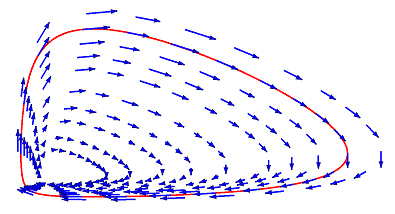
The vectors here are tangent vectors at flows through the phase space of possible solutions, i.e., represent the same linear approximations that occur in Taylor series. The linear term in Taylor series is a vector expression in the one-dimensional case, too, just less obvious. The use and significance of vector fields as tangent fields of continuous transformation groups in modern physics up to quantum field theory became unavoidable at the latest with the work of Lie and Noether at the end of the nineteenth and beginning of the twentieth century. The analysis of vector fields of dynamical systems like predator-prey systems, SIR models of pandemics (susceptible-infected-removed), etc., leads to the investigation of attractors, repellors, periodic, and chaotic trajectories.

Eigenvalues

Linear algebra, the theory of vector spaces, has the motivation to ask for repetitions or the absence of them in common with those phenomena. This means in the case of linear transformations that we ask for vectors that do not change direction (or at most are mirrored) by the application of a linear transformation
$$
\vec{v} \stackrel{\varphi}{\longrightarrow } \lambda\cdot \vec{v}.
$$
It is probably the most important challenge in linear algebra to find as many eigenvalues and eigenvectors of linear transformations as possible.

“The general concept of the eigenvalue of an endomorphism appeared in the eighteenth century [e.g. Legendre, 1762], not in connection with linear transformations, but in the theory of systems of homogeneous linear differential equations with constant coefficients. … In 1774 he [Lagrange] came across an analogous system in the theory of the “secular inequalities” of the planets, and Laplace also investigated this problem in 1784. … In the case of mechanical systems that depend on an infinite number of parameters, such as vibrating strings, the relationship between the problem of determining these frequencies and what we now call the spectrum of a second-order linear differential operator was already anticipated by D. Bernoulli; he arrived at the equation of the vibrating string by crossing a limit, starting from the movement of a finite number of masses that are equidistantly distributed on the string. Mathematically, however, the general concept of the eigenvalue of an operator in analysis only appeared with the theory of Sturm-Liouville.” [1]

This is another example of how mathematical concepts were developed in parallel with the treatment of problems in physics. It was only in the last century that mathematics developed more and more into a scientific field in which purely mathematical ideas were investigated.

The use of the prefix “eigen-” for characteristic quantities in this sense can be traced back to a publication by David Hilbert from 1904 in which he investigated linear integral equations and introduced the term eigenfunction. I cite Hilbert’s original text before its translation because it documents the origin of a technical term that is so widely used nowadays.

“Insbesondere in dieser ersten Mitteilung gelange ich zu Formeln, die die Entwicklung einer willkürlichen Funktion nach gewissen ausgezeichneten Funktionen, die ich Eigenfunktionen nenne, liefern: es ist dies ein Resultat, in dem als specielle Fälle die bekannten Entwicklungen nach trigonometrischen, Bessel’schen, nach Kugel-, Lamé’schen und Sturm’schen Funktionen, sowie die Entwicklungen nach denjenigen Funktionen mit mehr Veränderlichen enthalten sind, wie sie zuerst Poincaré bei seinen Untersuchungen über gewisse Randwertaufgaben in der Potentialtheorie nachwies.” [4]

“In particular, in this first notification I arrive at formulas which provide the expansion of an arbitrary function according to certain specific functions, which I call eigenfunctions: this is a result which contains, as special cases, the well-known expansions according to trigonometric, Bessel, spherical, Lamé and Sturm functions, as well as the expansions according to those functions with more variables, as first demonstrated by Poincaré in his investigations into certain boundary value problems in potential theory.”

Quantum Mechanics

Linear structures don’t only play a role as natural representation spaces, tangent spaces, in quantum field theory, they already occurred in early works of quantum mechanics. Heisenberg published in 1925 a paper about matrix mechanics that dealt with matrix representations of Hilbert spaces and operators on this Hilbert space to describe quantum mechanics, the Heisenberg formalism.

“The aim of this work is to provide a basis for a quantum theoretical mechanics that is based exclusively on relationships between fundamentally observable quantities.” [5]

Just one year later, in 1926, Schrödinger published his version of quantum mechanics, which was actually more classical in structure, studying wave functions and fluid mechanics. Schrödinger investigated the eigenvalue equation
$$
\hat H \psi=E\psi
$$
and commented

“I hope and believe that the above approaches will prove useful for explaining the magnetic properties of atoms and molecules and also for explaining the flow of electricity in solid bodies. There is undoubtedly a certain degree of difficulty in using a complex wave function at the moment. If it were fundamentally unavoidable and not just a calculation simplification, it would mean that there are basically two wave functions that only together provide information about the state of the system. This somewhat unpleasant conclusion allows, I believe, the much more sympathetic interpretation that the state of the system is given by a real function and its derivative with respect to time. The fact that we cannot yet provide any more precise information about this is due to the fact that in the pair of equations (4”) we only have the surrogate of a real wave equation of probably fourth order – which is admittedly extremely convenient for calculations – but I was unable to formulate it in the non-conservative case.” [6]

Schrödinger could show that his formalism is equivalent to Heisenberg’s. He introduced this result with an interesting comment.

“Given the extraordinary difference in the starting points and concepts of Heisenberg’s quantum mechanics on the one hand and the theory recently outlined here in its basic features and referred to as undulatory or physical mechanics on the other, it is quite strange that these two new quantum theories agree with each other with regard to the specific results that have become known so far, even where they deviate from the old quantum theory. I mention above all the peculiar half-integer nature of the oscillator and the rotator. This is really very strange, because the starting point, concepts, method, the entire mathematical apparatus seem to be fundamentally different. Above all, however, the departure from classical mechanics in the two theories seems to take place in diametrically opposite directions. In Heisenberg’s theory, the classical continuous variables are replaced by systems of discrete numerical quantities (matrices) which, depending on an integer index pair, are determined by algebraic equations. The authors themselves describe the theory as a true discontinuity theory. Undulation mechanics, on the other hand, represents a step from classical mechanics towards continuum theory. Instead of the event that can be described by a finite number of dependent variables using a finite number of total differential equations, there is a continuous field-like event in configuration space that is governed by a single partial differential equation that can be derived from an action principle. This action principle or differential equation replaces the equations of motion and the quantum conditions of the older classical quantum theory. In the following, the very intimate internal connection between Heisenberg’s quantum mechanics and my undulation mechanics will be revealed. From a formal mathematical point of view, this can probably be described as an identity (of the two theories).” [7]

Multiplications

Vector spaces carry often a second, multiplicative, distributive structure, i.e. constitute an algebra. Functions can be multiplied or folded, operator algebras which generalize matrix algebras, vector fields allow a Lie multiplication that obeys the Leibniz rule, Clifford algebras generalize Hamilton’s division algebra of quaternions, and biology knows genetic algebras. But we don’t need to define a separate structure. The vector space structure itself allows a multiplication which is quite important in physics and in mathematics, the tensor algebra of a vector space.

Tensor algebras evolved from the concept of duality, i.e. the observation that a vector can simultaneously be viewed as a linear form. Applying the same idea to bilinear and multilinear forms naturally leads to the concepts of tensor product and tensor.

“The symbolic method of invariant theory was thus brought to deal with two kinds of vectors in the same space, depending on whether they were transformed in one way or the other by a linear substitution, and which were distinguished by being called contragredient [contravariant] and cogredient [covariant], respectively.” [1]

This perspective is still crucial to the understanding of tensors in physics and also a bit confusing since mathematicians use the words co- and contravariant differently. Tensor algebras have an incredibly important property from a mathematical point of view, the universal property:

For any given bilinear transformation
$$\beta\, : \,\mathbb{R}^n\times \mathbb{R}^m\longrightarrow V$$
exists a uniquely determined linear transformation
$$\hat\beta\, : \,\mathbb{R}^{nm}\longrightarrow V$$
such that
$$
\beta=\hat\beta \circ \otimes .
$$
It means that we can turn a multilinear transformation defined on the Cartesian product of vector spaces into a linear transformation of a single vector space, the tensor algebra. A prominent example of the universal property is the Graßmann (exterior) algebra. It can be written as a quotient algebra, i.e. a surjective image of the tensor algebra
$$
\wedge V = \otimes V/\operatorname{span}\{ v\otimes v \}.
$$
It means that we define a multilinear, i.e. distributive structure on the Cartesian product of vector spaces of finite but arbitrary lengths, and impose the rule that any element vanishes that repeats an entry.

“Grassmann’s views go much deeper than Cayley’s. His great idea, which took shape in the discovery of the exterior algebra, was to develop a geometric analysis that goes much further than Möbius’s and calculates with extensive quantities. However, vectors in Cayley’s sense are only first-order quantities, whereas Grassmann wanted to introduce extensive quantities of any order and therefore could not be satisfied with this primitive standpoint. Looking back at history, we see him struggling to elaborate the abstract concept of the structure of vector space without fully succeeding. In the first edition (1844) of his major work, “Die Ausdehnungslehre” (The Theory of Extension), the fundamental concepts were not clearly defined and were linked to philosophical considerations that did not facilitate understanding. When he published a new, revised edition of this book in 1862, he was already much closer to his goal: the concepts of linear combination of linearly independent quantities, the basis of a domain (domain corresponds to our concept of vector space or vector subspace), and dimension are described very clearly; there, too, one finds for the first time the fundamental relationship between the dimensions of two vector subspaces:”
$$
\operatorname{dim} V +\operatorname{dim} W = \operatorname{dim}(V+W) + \operatorname{dim} (V\cap W).  [1]
$$
Graßmann algebras occur as the framework for oriented volumes as well as in algebraic topology, or as the algebra of differential forms, all of which are important in physics. Of course, these examples aren’t ultimately any different. There is a deep connection between volumes, differential forms, and the boundary operators in homology theory. Even the historical process reflects the fact that these connections aren’t obvious:

“The Graßmann algebra was only gradually rescued from oblivion when H. Poincaré and especially E. Cartan demonstrated its fundamental importance in differential geometry, and only after 1930, when E. Cartan’s work began to be understood, did Grassmann’s work again assume the central place it deserves in all applications of linear and multilinear algebra.” [1]

______________________________

“Symmetrical equations are good in their place, but ‘vector’ is a useless survival, or offshoot from quaternions, and has never been of the slightest use to any creature. Lord Kelvin.” [8]

Sources